Pharmakeyboard_arrow_rightWhite Papers / Preliminary results of predictive maintenance algorithms on a tablet press production machine.
menu

Federica Giatti, Compression Technologist at IMA Active Fabriano Ferrini, Product Manager for tablet presses at IMA Active |
Maintenance in automatic machines is usually addressed on a time basis. This means that parts are checked or substituted at regular time intervals or at a predetermined amount of working hours. This approach is called “pre-emptive maintenance”. In order to minimize the risk of a failure occurring before maintenance and thus unscheduled machine stops, system designers usually recommend intervention times shorter than the average time between failures. Therefore, although effective, the pre-emptive approach will generate a certain degree of wasted time and resources.
An alternative approach, called “predictive maintenance”, suggests performing maintenance only when necessary. In order to do it one must have a way to measure or estimate the state of health of the system and, if possible, an algorithm to predict the remaining useful life of the component. The two main benefits of such an approach are the optimization of resources and the possibility to schedule maintenance activities according to production needs.
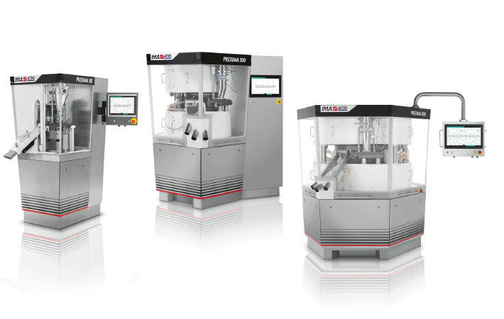
The subject of this study is a tablet press with several moving parts. Those parts require a proper balance of lubrication: too little lubricant can generate stress and early failures while too much can lead to other problems, among which the risk of leaking into the final product. Our goal was to be able to estimate the status of the moving parts with the following requirements:
• be integrated in the machine control system,
• run in real time,
• use the sensors already installed in the machine,
• be a self-teaching system, i.e. human intervention should be as limited as possible.
We performed the data collection by running the machine for several hours with no lubrication, until one of the moving parts reached failure. Two sensors were logged with a sampling rate of 10 kHz, for a total used disk space greater than 2 GB. Subsequently, the acquired data were used to train a machine learning classification algorithm through MATLAB tools. Figure 1 shows an example of the acquired signal.

Figure 1: first second of acquired signal.
The data from each sensor were divided into several segments of a fixed time length. We assigned a label to each segment ranging from 0 (perfect working condition) to 4 (failure in less than 30 minutes). An example is shown in Figure 2, with 600+ segments of 30 seconds each.

Figure 2: wear class subdivision of experiment.
Machine learning models usually do not accept time series as input; instead, they match several extracted features of a time series to a single output, in this case a predicted class. Deciding which and how many features to use is one of the most time-consuming tasks when designing a solution based on machine learning. To help us facilitate the process, we used an add-on integrated in the “Predictive Maintenance Toolbox” called “Diagnostic Feature Designer app”. We imported the waveform segments with their associated label and the app was able to generate 13 features in the time domain for each sensor. The app also had the capability of generating Power Spectrum Distributions, and then extract features in the frequency domain. We selected 5 characteristics, reaching 18 features per sensor, and 36 overall.
The extracted features are summarized in Table 1.
| Feature | Domain | Feature | Domain |
| Mean | Time | Clearance Factor | Time |
| Standard Deviation | Time | Signal-to-Noise Ratio | Time |
| RMS | Time | SINAD | Time |
| Shape Factor | Time | Total Harmonic Distortion | Time |
| Kurtosis | Time | Frequency of 1st peak | Frequency |
| Skewness | Time | Height of 1st peak | Frequency |
| Peak Value | Time | Frequency of 2nd peak | Frequency |
| Impulse Factor | Time | Height of 2nd peak | Frequency |
| Crest Factor | Time | Integrated band power | Frequency |
Table 1: feature list.
Among the selected features, some have a strong correlation with the label and carry the most information, others, on the contrary, are only weakly correlated to the classification class and are therefore less useful. The add-on provides a ranking of the extracted features based on one-way ANOVA. The full ranking is shown in Figure 3.

Figure 3: full ranking of all 36 extracted features.
Despite being extremely useful, the ranking lacks a fundamental information: not all the entries are independent; pairs of features can have strong correlation factors, which means that the amount of information they carry is similar, if not identical. The extreme case is the triplet Mean, RMS and Standard Deviation that are linked by a mathematical equation (RMS2 = Mean2 + StdDev2).
It is not a coincidence, in fact, that they have a similar rank. In order to select a small set with only the most meaningful features we used three different approaches:
1. Manual choice
2. Correlation Matrix sieve
3. Neighbourhood Component Analysis (NCA)
We picked the features we thought were the most useful based on the knowledge of the system. We selected a total of 6 features: Mean, Standard Deviation and Band Power for each sensor.
We calculated the correlation matrix of all the 36 features. We then started looking at the ranking from top to bottom. We picked the highest ranked and eliminated all those having a correlation coefficient greater than 0.7. Among the remaining, we picked the second highest and repeated the process until we picked a total of 5 features. The resulting set was composed of: Mean, Shape Factor and Band Power of sensor 1, Mean and Band Power of sensor 2.
Neighbourhood Component Analysis is a technique used for automatic feature selection. It takes as input K eatures for N entries and the corresponding N labels and produces K output values, one per feature. The output can be interpreted as an “importance factor” immune to correlation. In practice, the output can be used to create a new ranking. Figure 4 shows the NCA output, with indication of the top 10 features.
We chose the top 5 features, namely Shape Factor of sensor 1 and Mean, Shape Factor, THD and Skewness of sensor 2.

Figure 4: Output of NCA algorithm with top 10 features highlighted.
We imported the data from the three defined subsets of features into the “Classification Learner” add-on in MATLAB.
The add-on can test several Machine Learning classifications. To avoid over-fitting we used 5-fold cross validation. For each subset we picked the algorithm with the highest accuracy and compared the three.
The three best confusion matrices are displayed in Figure 5. It can be seen that all three subsets achieved classification accuracies well above 85%. The manual choice set is the least accurate with 87% whereas the two other methods of feature selection achieved a slightly higher accuracy: 89%. What makes the two automatic selection methods more appealing is not only the better accuracy, but also the fact that they work with a smaller dimensionality. As a general rule, in fact, the lower the dimensionality, the higher the chances are that the Machine Learning model can generalise and deliver good results with data different from the training ones. Between the correlation and NCA we picked the latter because it has a slightly better accuracy when the true class is 4, the class indicating an imminent failure.

Figure 5: confusion matrices for the three tested subsets of features.
We were able to use the sensors already installed in the machine to obtain additional information for the estimation of the state of health of some critical moving parts. We logged the sensors’ data while running the machine without lubrication until one part reached failure. We divided the full time series into segments and assigned them a label indicating the status of the moving part. Subsequently, we used MATLAB’s “Diagnostic Feature Designer” app to automatically extract and select the features that best correlate with the status. Finally, we built a Machine Learning classification model that achieved 89% classification accuracy using only 5 extracted features.